In computer science, the Big-O notation is used to describe the performance or complexity of an algorithm relative to the size of the input. In other words: what happens to the performance/complexity of an algorithm when its input gets arbitrarily large? Big-O, with respect to other notation types, specifically describes the worst-case scenario of this performance.

What's the Big(-O) deal?

Why is it important to understand Big-O notation? Before we can answer that, let's start out with a little background about efficiency, performance and complexity of algorithms.

Efficiency of an algorithm covers lots of resources, including:

CPU (time) usage
memory usage
disk usage
network usage

All are important but we will mostly talk about time complexity (CPU usage). In this context, it is important to differentiate between:

Performance - how much time/memory/disk/etc. is actually used when a program is run. This depends on the machine, compiler, etc. as well as the code.
Complexity: how do the resource requirements of a program or algorithm scale. In other words: what happens as the size of the problem being solved gets larger?

Complexity affects performance but not the other way around.

Since Big-O notation tells you the complexity of an algorithm in terms of the size of its input, it is essential to understand Big-O if you want to know how algorithms will scale.

The Big-O notation itself will not help you. Rather, understanding Big-O notation will help you understand the worst-case complexity of an algorithm. Essentially, Big-O gives you a high-level sense of which algorithms are fast, which are slow and what the tradeoffs are.

Introductory example

Consider a magical, but inefficient and heavy, traditional paper phone book in which each page contains the details of only one person. We want to find the page on which a person's details are written. There are several methods (algorithms) of doing this. We will analyse the following two algorithms as an introductory example:

Start at page 1 and sequentially browse through every page until the person we're looking for is found.
Start half-way the phone book, look at the name of the person on the page and decide whether the person we're looking for is alphabetically in the first or the second half of the book. Then open the phone book in the middle of the chosen half and make the decision again. Rinse and repeat until the page with the requested person is found.

For a phone book with just a few pages (small input), the difference in performance between the above examples may be relatively small. However, for large phone books with many pages (arbitrarily large input) the difference in performance is huge.

Best case, the first algorithm requires only 1 lookup if the person we're looking for is on the first page of the phone book. Worst-case however, the situation we consider for the Big-O notation, it would require going through all entries in the phone book when we're looking for ZZ Top for example. Let's take a look at the performance of both algorithms.

Algorithm 1 - incremental browse

Let the number of people in the phone book be \(n\). The number of operations for the algorithm in the first example increases by 1 for every person added to the phone book. This means that worst-case we would need to browse through \(n\) (all) entries to find our match. This classifies this algorithm as linear, or in Big-O notation as \(O(n)\); we state this algorithm has an order of n.

Algorithm 2 - binary search

The second algorithm uses a binary search approach to find a match: with each operation we halve the problem space. This means that each time we double the amount of pages in the phone book, the amount of operations to find our match increases by 1. This classifies this algorithm as logarithmic, or in Big-O notation as \(O(log\ n)\); we would say this algorithm has an order of log n.

Note that when evaluating complexity of algorithms, constants are not taken into account because they do not significantly affect the number of operations (when \(n\) gets really big). An algorithm which does \(n\) steps and algorithms which do \(2n\) or \(n/3\) respectively are still considered linear (\(O(n)\)) and approximately equally efficient.

Now let's take a look at a few other examples of the Big-O notation.

Big-Order of magnitude

A number of very common order of magnitude functions will come up over and over as you study algorithms. These are shown in the following list and will be covered in this article:

Constant - \(O(1)\)
Logarithmic - \(O(log\ n)\)
Linear - \(O(n)\)
Log Linear - \(O(n\ log\ n)\)
Quadratic - \(O(n^2)\)
Exponential - \(O(2^n)\)
Factorial - \(O(n!)\)

Before diving into details of each classification, let's see how these categories perform relatively when their input gets really large.

Performance comparison

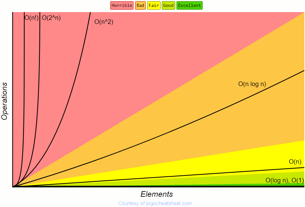
The chart below depicts the Big-O complexities mentioned above and the number of elements in the input against the number of operations. The color coding provides a rough judgement on their performance.
bigochart

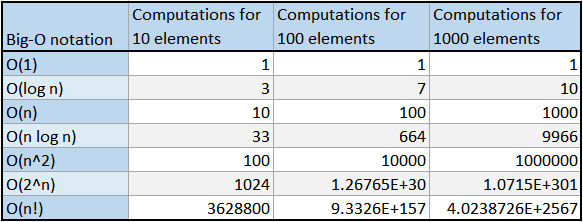
The table below shows just how big of a difference the number of computations between these algorithms are for 10, 100 and 1000 input elements:
bigoperformance-2

Bonus trivia: It takes Siri almost 13 minutes to pronounce the numbers in 1000!

Constant - \(O(1)\)

\(O(1)\) describes an algorithm that will always execute in the same (constant) time (or space), regardless of the size of the input data set.

An example is the code that returns whether a number is even or odd, like in the following C# code:

public bool IsEven(int number)
{
   return number % 2 == 0;
}

Logarithmic - \(O(log\ n)\)

Algorithms with an order of log n generally reduce the problem size with each operation. The most common attributes of these algorithms are that:

the choice of the next element on which to perform some action, is one of several possibilities, and
only one of these possibilities will need to be chosen.

In the introductory example, the second algorithm repeatedly splits the (remaining) pages of the phone book in two halves. Depending on the half in which the target person is in, one half is chosen and the other half discarded.

An example of a snippet of C# code with an order of log n is the following:

while (n > 1)
{
   n = n / 2;
}

Other examples of log n algorithms are:

Binary Search
Finding the largest/smallest number in a binary tree

Linear - \(O(n)\)

\(O(n)\) describes an algorithm whose performance will grow linearly and in direct proportion to the size of the input data set. In the introductory example, the first algorithm required looping through every single entry of a phone book until the match was found, thus having an order of n.

The following example in C# also has an order of n and loops through a list of elements until a given value is found:

public bool Contains(IList elements, int value)
{
   foreach (var element in elements)
   {
      if (element == value)
         return true;
   }
   return false;
}

Other examples of linear algorithms are:

Finding the min/max element in a list
Iteratively finding the nth Fibonacci number

Log linear \(O(n\ log\ n)\)

Algorithms with \(O(n\ log\ n)\) perform a \(O(log\ n)\) operation for each item in the input.

Most efficient sort algorithms fall under this category, like Merge Sort, Heap Sort and Quick Sort. Another example of a \(O(n\ log\ n)\) algorithm is the Fast Fourier Transform.

Quadratic - \(O(n^2)\)

\(O(n^2)\) describes an algorithm whose performance will grow linearly and in direct proportion to the size of the input data set squared.

Where a linear (\(O(n)\)) example would be a loop through all n elements of a list, a quadratic example is a double nested loop. More practical, most inefficient sort algorithms fall under this category, like Selection sort, Insertion sort and Bubble sort, as we will see below.

Bubble sort

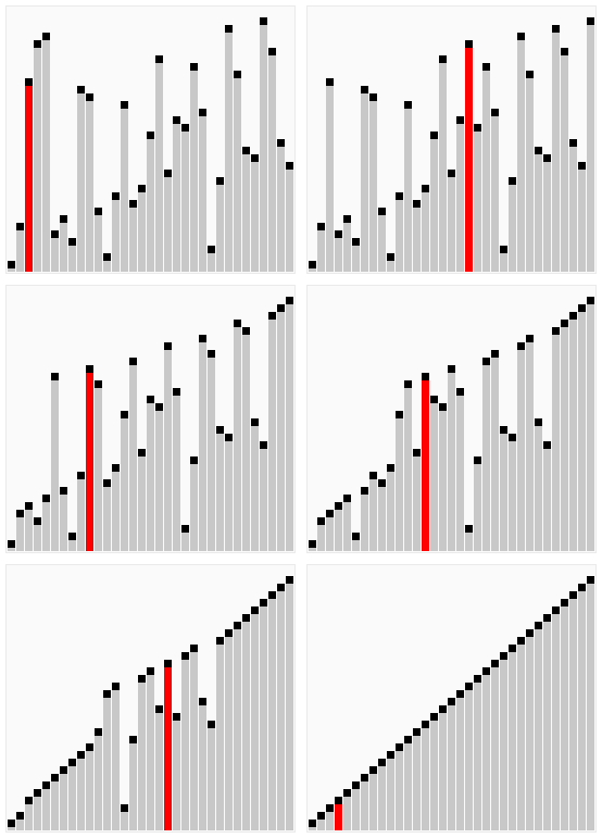
The Bubble sort algorithm repeatedly iterates the input container to be sorted, compares each pair of adjacent items and swaps them if they are in the wrong order. It continues to do so until no swaps were made, indicating that the list is sorted. By doing this, the bigger items 'bubble' up, hence the name 'Bubble sort'. See the animation below for an example.

Bubblesort

The following code is an implementation of the Bubble sort algorithm in C#:

public void BubbleSort(int[] input)
{
    bool hasSwapped;
    do
    {
        hasSwapped = false;
        for (var sort = 0; sort < input.Length - 1; sort++)
        {
            if (input[sort] > input[sort + 1])
            {
                var oldValue = input[sort + 1];
                input[sort + 1] = input[sort];
                input[sort] = oldValue;
                hasSwapped = true;
            }
        }
    } while (hasSwapped);
}

The outside 'do - while' loop (line 4 - 17) worst case makes n passes for an input in which the elements are in reverse sort order, making this loop do \(O(n)\) work.
The inner 'for'-loop (line 7 - 16) also runs in order of n. n - 1 to be precise, however we discard the constant because it is less significant when n gets really big (see the notes in the introductory example).

Note: Any algorithm that has a complexity of \(O(n^a)\), with \(a\) is a non-negative integer, is said to have polynomial complexity or is solvable in polynomial time.

Exponential - \(O(2^n)\)

\(O(2^n)\) complexity is an algorithm whose growth doubles with each additon to the input data set. With small inputs the growth curve is very small, but it rises exponentially when the input gets larger.

An example of an exponential algorithm is the recursive calculation of the n-th Fibonacci number, like in the C# example below:

public long Fibonacci(int number)
{
   if (number <= 1)
      return number;

   return Fibonacci(number - 1) + Fibonacci(number - 2);
}

Factorial \(O(n!)\)

\(O(n!)\) represents an algorithm which has to perform n! computations to solve a problem. These algorithms take a massive performance hit for each additional input element. For example, an algorithm that takes 2 seconds to compute 2 elements, will take 6 seconds to calculate 3 and 24 seconds to calculate 4 elements.

Traveling Salesman Problem

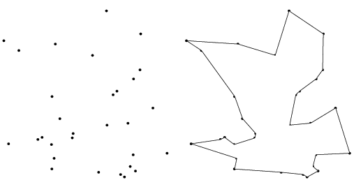
One famous problem in Computer Science is the Traveling Salesman Problem (TSP). In this problem there are n cities. Each of these cities is linked to 1 or more other cities by a road of a certain distance. The TSP is to find the shortest tour that visits every city.

TravelingSalesmanProblem_1000

Deceptively easy.

Consider the scenario in which we have 3 cities A, B and C. These are the possible combinations with roads connecting all cities and returning to the starting-point:

A - B - C - A
A - C - B - A
B - A - C - B
B - C - A - B
C - A - B - C
C - B - A - C

When we take a closer look at these results, all possibilities are the same route with a different starting point or in reverse. So, when we remove equivalent routes we end up with 1 unique route for an input of 3 cities:

A - B - C - A

tspabc

If we increased the number of cities to 4, we end up with 3 possible routes, with 5 cities 12 routes, with 6 cities 60 routes and with 7 cities 360 possible routes. Bonus note: The number of possible routes is \((n-1)!/2\) for \(n >= 3\).

These results are a mathematical function called factorial, which outputs as shown below:

3! = 3 x 2 x 1 = 6
4! = 4 x 3 x 2 x 1 = 24
5! = 5 x 4 x 3 x 2 x 1 = 120
10! = 10 x 9 x ... x 2 x 1 = 3,628,800
25! = 25 x 24 x … x 2 x 1 = 15,511,210,043,330,985,984,000,000
50! = 50 x 49 x … x 2 x 1 = \(3.04141*10^{64}\)
200! = really, really big

The complexity of the Traveling Salesman Problem is \(O(n!)\).

Bonus trivia: If each computation would take 1 millisecond and we would have started all calculations at the moment of the Big Bang, we would have finished calculating 21 cities 12 billion years ago. It will still take an extra 22 billion years for the calculation of 22 cities to finish.

Understanding Big-O notation